Enthalpy of solution calculations

This post will discuss how to approach enthalpy of solution calculations. This is in Module 4 of the current NSW Stage 6 curriculum, and as such is assumed knowledge but not directly examinable in the HSC. So in some sense, agreeing upon one method to use internally in your teaching and assessments (e.g. the one your textbook uses) is a good way to go.

That having been said, we can estimate the heat capacity (=mass × specific heat capacity) of a solution in the following ways (there are also others):

1. Measure it directly (e.g. measure masses and make solution of desired concentration, then transfer a known amount of energy and measure temperature change). This is possible but fairly impractical.

2. If you know the mass and specific heat capacity of both the solute and solvent (e.g. water), then the heat capacity of the solution can be estimated as m(water) × c(water) + m(solute) × c(solute)

Generally we can’t (or aren’t) doing either of those, so we need more approximate methods. For example:

3. We can assume that the salt contributes to the overall heat capacity of the solution identically to water, i.e. the heat capacity of the solution = m(solute) × c(water) + m(water) × c(water). This will overestimate the heat capacity of the solution, as c(solute) < c(water) for most (all?) ionic solutes.

4. We can assume that the salt contributes nothing to the overall heat capacity of the solution. i.e. the heat capacity of the solution = m(water) × c(water). Effectively we are assuming that m(solute) × c(solute) = 0, so this will underestimate the heat capacity of the solution. The following graphs demonstrate this for the three salts that my class used for this practical this year: sodium hydroxide, potassium nitrate and ammonium chloride (the NaOH graph also has some literature data). Blue dots are method 2, grey dots are method 3, orange dots are method 4. As can be seen in the graphs, the value from method 2 is in between the values from methods 3 and 4, but method 4 always gives the better approximation. This is because c(water) is usually much larger than c(solute) for an ionic solute, and m(solute) is usually relatively small compared to the m(water). In such cases, m(water) × c(water) >> m(solute) × c(solute), so the assumption that m(solute) × c(solute) = 0 isn’t a terrible one.

Generating MCQ response graphs with ImageJ

Introduction

I find graphs of multiple choice question response data very useful in analysis of misconceptions, so I developed a procedure to rapidly (i.e. within 10 min) generate such graphs with freely available software and minimum user input. It does, however, rely on being able to rapidly scan large numbers of papers quickly (e.g. using the scan and send function on a photocopier).

MCQ-summary

Basically the process goes like this:

  1. Scan MCQ papers and manipulate such that you end up with a folder of low-resolution images.
  2. Use ImageJ (and plugins) to load these image files and for each question, read the lightness/darkness of each choice bubble (i.e. has it been coloured in or not).
  3. Peform calculations and generate graphs from this data using a spreadsheet.

Required software

You will need access to the following software:

  • Spreadsheet program (Excel or equivalent)
  • ImageJ (download the appropriate version and install)
  • MicroArray Profile plugin for ImageJ (download and extract to the ImageJ plugins folder)
  • The analysis spreadsheet: microarray profile-graphs.xlsx
  • If you wish to try the rest of the process out you can download this zip file, which contains some sample MCQ scans: MCQsample.zip

1. Scan MCQ papers

I am very fortunate to have access to a photocopier that will feed and scan multiple documents rapidly and then email the resulting pdf to you.

I take about 20 MCQ sheets at a time and make sure they’re lined up with each other, then place in the document feeder (the alignment has to be pretty good; you want the same choice bubbles in the same place on each scanned page). Repeat as required, then scan. If you have a large number of papers (> 120) you may wish to do this in a couple of batches. Scanning takes me a couple of minutes for 180 papers.

2. Export pdf pages to image files

Open the pdf and in Acrobat choose File – Export – Image – JPEG (or whatever you need to do to get to a stage where each paper has been scanned to an individual image file) and save them to a blank folder.

export pdfWhen you need to choose JPEG settings, I use the following (96 pixels/inch is enough). You can use higher quality files if you like, but it’s not super necessary and it can hog a lot of memory when you import them into ImageJ in the next step.

jpg settingsIf you wish to try the rest of the process out you can download this zip file, which contains some sample MCQ scans: MCQsample.zip

3. Import image files into ImageJ

Open ImageJ, and File – Import – Image Sequence and select the first image file you generated in step 2. You will be prompted to import the files, hit OK.

import image sequence4. Rotate and crop images (optional, but recommended)

I usually rotate and crop images in order the facilitate placing the grid (step 5). My spreadsheet is set up for images rotated 90 degrees left, i.e. top of the page facing left). To rotate, Image – Transform – Rotate 90 degrees left. To crop, select the area you wish to crop with the rectangle tool (selected by default) then Image – Crop (or Ctrl + Shift + X). Zoom to your desired size so the image takes up most of the screen.

rotate5. Set the Microarray Profile grid

Select Plugins – Microarray Profile, then select the “Reset Grid” button from the MAP window that appears. Input the number of choice bubbles per question in “Rows” and the number of questions in “Columns”. In this example, there are 14 MCQ, each with 4 choice bubbles (A through D).

grid0A grid of yellow circles will be placed over the choice bubbles, as you can see in the picture above.

  1. If the grid of circles is much bigger than the grid of bubbles, Shift-drag a corner circle to shrink the grid to approximately the right area (in this case I shift-dragged the top right circle).grid1
  2. Alt-drag a corner circle so that it aligns with the corresponding corner choice bubble in the image (in this case, I alt-dragged the bottom right circle to Q14 A).grid2
  3. Shift-drag an adjacent corner circle so that it is positioned properly. Now the whole edge connecting the two corners should be lined up with the spots (in this case, I shift-dragged the top right circle; now the Q14 circles all line up).grid3
  4. Shift-drag a spot in the interior of the opposite edge until that edge is lined up with the spots (in this case, I shift-dragged the circle corresponding to Q1 B).grid4
  5. All of the circles should now be aligned more or less aligned with the spots. You can drag any individual circle to adjust its position independently of the other circles.
  6. (Optional) Scroll through the a few images to verify that the grid placement is correct for these images.

6. Read histogram and save results

Select the “Histograms” button from the MAP panel and wait patiently. When the results window pops up, select File -> Save As and save the file somewhere sensible (the default filename is Results.xls).save as7. Import data into spreadsheet

  1. Open microarray profile-graphs.xlsx. Select cell A1 of the ‘microarray‘ worksheet.microarray sheet
  2. Open Results.xls (that you exported in step 6 above). Excel will have a whinge at you that it’s not in the correct format; ignore it and select Yes.error
  3. Select and copy all of the data in Results.xls (Ctrl + A, Ctrl + C). The top left of the sheet will look like this:Results
  4. Paste this data into the ‘microarray‘ worksheet of microarray profile-graphs.xlsx.

8. Set black/white threshold

  1. The data in column I (Mean) is the mean value assigned by ImageJ (where 0 = black and 255 = white). We need to pick a black/white threshold value so that coloured-in bubbles have mean values below the threshold, and blank bubbles have mean values above the threshold. Eyeball the data in the ‘microarray‘ worksheet, compare with the image files in ImageJ, and decide on a black/white threshold value (for my exam papers it’s usually somewhere between 170 and 210 depending on paper and scanning settings).
  2. Select the ‘summary data‘ worksheet. Adjust the black/white threshold value, if required (cell T1).summary data

And that’s it! The results are now displayed in the ‘summary data‘ worksheet, and graphically in the ‘Graph *‘ worksheets.

Restrictions and limitations

The one major limitation is that choice bubbles coloured-in and then crossed out will be counted as coloured-in. For example, question 4 for the paper below will be counted as having both A and B coloured-in:

save asThe only realistic way around this is to make students erase any incorrect responses. As it stands, though, this can actually provide some extra feedback on useful distractors even if the correct answer is ultimately selected.

I hope this was of use, please leave a comment if you have any suggestions for further improvement!

Cheryl’s precipitate

Albert and Bernard just became friends with Cheryl, and they now know when her birthday is! They see that she is holding a test tube containing a solution and a precipitate, which she tells them that she has produced by mixing two 0.02 M aqueous solutions. They want to know what precipitate she has produced. Cheryl gives them a list of possible cations and anions present in the original solutions: Na+, Ag+, Ba2+, Mg2+, OH, CO32–, Cl, SO42–. She tells Albert the identity of the anion present in the precipitate and Bernard the identity of the cation present in the precipitate.

Albert: I don’t know what the precipitate is.

Bernard: I didn’t, but now that you’ve said that, I do.

Albert: Then so do I.

What is the precipitate?

#cherylsprecipitate

Marking philosophy

Michael Seery has posted an interesting summary and discussion of this paper on grading practices, specifically showing working/reasoning. Go read both if you haven’t already, but here’s a TL;DR question: if a student gets the correct answer to a question, do they automatically get full marks or do they need to show their working/logic? Another way of looking at it is this: does the burden of proof lies with the student or the examiner?

Philosophically, students showing their working is something I want to encourage, as it is good for them (makes clear the sequence of logical steps taken, makes checking/reflecting on their work easier) and makes a marker’s life easier (important in the context of exams).

As a test case, consider a student who gets the correct answer using an incorrect method (e.g. two mistakes cancelling each other out, or a correct choice made for incorrect reasons). This will be obvious if they show their working, but not if they don’t. In this scenario above, penalising the student only when they show their (incorrect) working has the effect of discouraging students from showing their working in the first place, so it’s not something I want to do. On the other hand, taking marks off for incomplete or missing working does seem a bit harsh if the student has in fact used the correct method!

My question setting/marking philosophy

My broader philosophy is that we should be looking to award marks for working/logic shown, not looking to take marks off for what is not shown. The difference is subtle, but I think the former is a better attitude. A corollary of this is that as an examiner, if you want to see something in an answer you should allocate a mark for it when you’re deciding how much the question is worth.

On the burden of proof question, my personal opinion is that the examiner should write questions such that there is no problem with the burden of proof lying on the examiner if the answer is correct, but that showing working is still encouraged by shifting the burden of proof to the student if their answer is incorrect.

1. Avoid error-cancelling

I try to avoid situations where numerically correct answers can be obtained by an incorrect method. This generally entails just using numbers that are not as nice and/or ensuring that dilution factors/aliquot volumes/concentrations don’t coincide or cancel.

2. Eliminate trivial steps or award marks only for non-trivial steps

As an example, consider the following question:

25.00 mL of 0.1012 M hydrochloric acid is required to neutralise 20.00 mL of a sodium hydroxide solution. Calculate the molar concentration of the sodium hydroxide solution. (3 marks)

For which my ideal working might go something like this:

HCl(aq) + NaOH(aq) ? NaCl(aq) + H2O(l)

n(HCl) = 25.00 mL x 0.1012 M = 2.530 mmol

n(NaOH) = 2.530 mmol

[NaOH] = 2.530 mmol / 20.00 mL = 0.1265 M

Conceptually the student has to take 3 logical steps (for 3 marks):

  1. Calculate n(HCl)
  2. Realise that n(NaOH) = n(HCl)
  3. Calculate [NaOH].

But consider a student who writes the following (quite common in my experience):

n(HCl) = 25.00 mL x 0.1012 M = 2.530 mmol

[NaOH] = 2.530 mmol / 20.00 mL = 0.1265 M

They have clearly done steps 1 and 3, but how can you be sure about step 2? Does the burden of proof lie on the student or teacher here (i.e. do you award them 2 marks or 3 marks)?

I would alter this question in one of two ways to avoid this problem:

  • Make the question out of only two marks and to award those marks for steps 1 and 3 (i.e. no marks awarded for taking the trivial step 2). This is not my preferred option, but it does keep the question easier.
  • Keep the question out of 3 marks and make step 2 non-trivial

e.g. use H2SO4 instead of HCl so the mole ratio is no longer 1:1 and change the NaOH volume to 10.00 mL:

25.00 mL of 0.1012 M sulfuric acid is required to neutralise 10.00 mL of a sodium hydroxide solution. Calculate the molar concentration of the sodium hydroxide solution. (3 marks)

For which my ideal working might go something like this:

H2SO4(aq) + 2NaOH(aq) ? Na2SO4(aq) + 2H2O(l)

n(H2SO4) = 25.00 mL x 0.1012 M = 2.530 mmol

n(NaOH) = 2 x 2.530 = 5.06 mmol

[NaOH] = 2.530 mmol / 10.00 mL = 0.506 M

Conceptually the student has to take 3 logical steps (for 3 marks):

  1. calculate n(H2SO4)
  2. realise that n(NaOH) = 2 x n(H2SO4)
  3. calculate [NaOH].

This shifts the burden of proof off the student: if I (as an exam setter) want to find out if a student can do something, I make sure they have to do it in order to get the right answer. I favour this course of action, as it also means that students who blindly apply the dilution formula (C1V1=C2V2) will not get the right answer.

If a student gets the correct answer then they must have performed all required steps, so I am comfortable with the burden of proof being on the examiner in this case.

The problem with this philosophy is that it doesn’t encourage or require working at all. Here’s the kicker though…

3. Award carry-through errors only if working is clear

So if a student gets the correct answer but with little/no working, they are awarded full marks. What if they don’t get the correct answer? This is where the exam-based reinforcement of all the intrinsically good reasons for showing your working/logic happens…

Got the wrong answer but showed all your working? You’ll be awarded marks for any step for which you have the correct working (regardless of previous errors). So for the example above,  if you show correct working for steps 1 and 3 but you miss the 2:1 ratio in step 2 (or apply it the other way around), then you will still be awarded marks for correctly performing steps 1 and 3.

Got the wrong answer and didn’t show clear, logical working? You’re out of luck, buddy.

I don’t have a problem with shifting the burden of proof onto the student in this case, as they’ve already demonstrated that they haven’t done at least one of the required steps.

What do you think? Where do you decide the burden of proof lies? Are you comfortable with the burden of proof shifting depending on whether the final answer is correct or not?

Creative Commons License

This work is licensed under a Creative Commons Attribution-NonCommercial-ShareAlike 3.0 Australia License

Titration curves

Introduction

After a recent discussion with a colleague I decided to investigate and write a post about the factors that influence the shape of titration curves. Acid-base titration curves (graphs of solution pH against volume of titrant added) will be discussed as these are the most common type encountered at high school, but much of what follows can be generalised to other types of titration. For a more in-depth analysis of these and other methods, Vogel’s Quantitative Chemical Analysis is a good place to start.

The shape of an acid-base titration curve has a direct influence on many aspects of a titration including titrant/titrand choice, indicator choice, whether an indicator is appropriate at all, or which equivalence point is easier to detect if there is more than one. The pH of an acid or base solution is affected by both the strength of the acid or base and its concentration, so it should be unsurprising that both of these affect the shape of an acid-base titration curve (n.b. strength is not the same thing as concentration, if you’re not sure about the difference it’s probably worth taking the time to sort that out before continuing).

High school students should probably be familiar with titration curves for monoprotic strong acid-strong base, weak acid-strong base, strong acid-weak base and possibly weak acid-weak base, all at concentrations around 0.1 M. These are presented in Fig. 1-4 below (generated with the wonderful CurTiPot).

monoprotic strong acid strong base BTB

Fig. 1: 0.1 M HCl vs 0.1 M NaOH

Features:

  • neutral equivalence point pH
  • very sharp change in pH either side of the equivalence point (the near vertical section from pH 4 to 10 at 25 mL)
  • can detect the equivalence point using e.g. bromothymol blue, as shown on the graph (yellow at pH 6.0, blue at pH 7.6)

monoprotic weak acid strong base PT

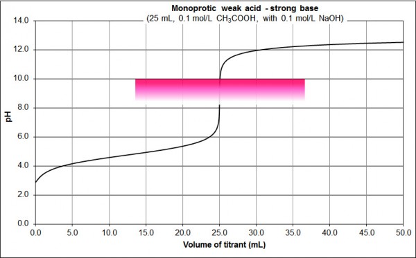
Fig. 2: 0.1 M CH3COOH vs 0.1 M NaOH

Features:

  • basic equivalence point pH
  • sharp change in pH either side of the equivalence point (the near vertical section from pH 8 to 10 at 25 mL, but contrast the pH change in this vertical region to that of Fig. 1)
  • can detect the equivalence point using e.g. phenolphthalein, as shown on the graph (colourless at pH 8.2, pink at pH 10.0)

monoprotic strong acid weak base MR

Fig 3: 0.1 M HCl vs 0.1 M NH3

Features:

  • acidic equivalence point pH
  • sharp change in pH either side of the equivalence point (the near vertical section from from pH 4 to 6 at 25 mL, but contrast the pH change in this vertical region to that of Fig. 1 and compare with Fig. 2)
  • can detect the equivalence point using e.g. methyl red, as shown on the graph (red at pH 4.4, yellow at pH 6.2)

monoprotic weak acid weak base BTB

Fig. 4: 0.1 M CH3COOH vs 0.1 M NH3

Features:

  • ~neutral equivalence point pH (depends on the relative strength of the weak acid and weak base)
  • gradual change in pH either side of the equivalence point (contrast Figs. 1-3)
  • difficult to detect equivalence point using conventional indicators as the colour change is gradual (alternatives include coulometric, thermometric or conductimetric titrations; use of mixed indicators; or simply titrating with a strong acid/base).

Acid/base strength effects: monoprotic acids and monobasic bases

As can be seen by comparing fig. 1 and 2 above, acid/base strength is one variable that affects the shape of titration curves.

The following graph shows the effect of acid strength on the shape of the titration curve. Acid strength can be measured by the acid’s pKa: smaller pKa = stronger acid, larger pKa = weaker acid.  All concentrations are 0.1 M (the effect of concentration will be investigated later).

pKa monoprotic acid

Fig. 5: 0.1 M monoprotic acids vs 0.1 M NaOH, pKa variation

Features:

  • The strongest acid (brown, pKa = -7, e.g. HCl) curve is as per Fig. 1 above; the pH changes rapidly either side of the equivalence point.
  • Successively weaker acids shift the pH of the equivalence point higher, and the pH change either side of the equivalence point is less pronounced.
  • The acetic acid (pKa = 4.76) curve, as per Fig. 2 above, would be between the lilac pKa =  4 and royal blue pKa = 5 curves.
  • The dark green pKa = 7 curve, representing an acid with a pKa of 7, has a rapid pH change of only about 1.5 at the equivalence point. This is about the limit for all but the sharpest indicators.
  • Weaker acids than this (i.e. the fluoro green pKa = 8 curve and above) only show a gradual change (if indeed any at all) in pH around the equivalence point.

A similar range of curves is found for the titration of the conjugate bases of these acids with hydrochloric acid (the pKa values indicated are for the parent acids, in the same order as in Fig. 5). Again, all concentrations are 0.1 M.

pKa monobasic base

Fig. 6: 0.1 M monobasic conjugate bases vs 0.1 M HCl, parent acid pKa variation

Features:

  • The order of strengths is effectively swapped
  • The conjugate bases of the weakest acids from Fig 5 (i.e. the fluoro green pKa = 8 curve and above) now show a sharp change in pH either side of the equivalence point.
  • The dark green pKa = 7 curve has a rapid pH change of only about 1.5 at the equivalence point. Again, this is about the limit for all but the sharpest indicators.

Acid strength effects: diprotic acids

Diprotic acids can give rise to quite different titration curves, depending on the absolute and relative strengths of each dissociation.

The following graph shows the different titration curves from acids with

  • a strong first dissociation: pKa1 = -3
  • variable second dissociation strength: pKa2 = 2 (pink curve), pKa2 = 7 (dark green curve) or pKa2 = 12 (black curve).

Again, all concentrations are 0.1 M.

pKa diprotic acid pKa1=_-3_pKa2, 7, or 12-0.1 M

Fig. 7: 0.1 M diprotic acid (pKa1 = -3, pKa2 = 2, 7 or 12) vs 0.1 M NaOH

Features:

  • Only one equivalence point (at 40 mL) is seen when both the first and second dissociations are strong (e.g. the pink pKa2 = 2  curve)
  • When the first dissociation is strong and the second moderately weak, it is possible to detect two equivalence points, one at 20 mL and one at 40 mL (e.g. the dark green pKa2 = 7  curve).
  • Only one equivalence point (at 20 mL) is seen when the first dissociation is strong and the second very weak (e.g. the black pKa2 = 12 curve).

The following is a similar graph with smaller pKa2 spacing:

pKa diprotic acid pKa1=_-3_pKa2=2-12

Fig. 8: 0.1 M diprotic acid (pKa1 = -3, pKa2 = 2-12) vs 0.1 M NaOH

Features are similar to Fig. 7:

  • Only one equivalence point (at 40 mL) is seen when both the first and second dissociations are strong (e.g. the pKa2 = 2 and pKa2 = 3 curves)
  • When the first dissociation is strong and the second moderately weak, it is possible to detect two equivalence points, one at 20 mL and one at 40 mL. Which one is sharper depends on the relative weakness of the second dissociation.
  • Only one equivalence point (at 20 mL) is seen when the first dissociation is strong and the second very weak (e.g. the pKa2 = 11 and pKa2 = 12 curves).

A similar effect is seen when the first pKa is weaker (e.g. pKa1 = 4):

pKa diprotic acid pKa1=4_pKa2=5-12

Fig. 9: 0.1 M diprotic acid (pKa1 = 4, pKa2 = 5-12) vs 0.1 M NaOH

Concentration effects: monoprotic acids

concentration monoprotic strong acid

Fig. 10: monoprotic strong acid, X M (pX = -1 – 5) vs X M NaOH

Features:

  • The lower the acid/base concentrations, the less pronounced the pH change either side of the equivalence point.
  • Somewhere between pX = 3 and 4 is about the limit for all but the sharpest indicators

For a weak acid similar features are observed, except that a higher concentration of acid and base is required to give an equivalent change in pH either side of the equivalence point. This makes sense given that the pH change either side of the equivalence point is already less pronounced for a weak acid than it is for a strong acid (compare Figs. 1 and 2).

concentration monoprotic weak acid

Fig. 11: monoprotic weak acid (pKa 4.76), X M (pX = -1 – 5) vs X M NaOH

Concentration effects: diprotic acids

concentration diprotic acid pKa1=_-3_pKa2=2

Fig. 12: X M diprotic acid (pX = -1 – 5, pKa1 = -3, pKa2 = 2) vs X M NaOH

Features:

  • As above, the lower the acid/base concentrations, the less pronounced the pH change either side of the equivalence point.
  • As above, somewhere between pX = 3 and 4 is about the limit for all but the sharpest indicators
  • At pX = -1 (i.e. a concentration of 10 M) the first equivalence point becomes detectable

Consider again Fig. 7 (0.1 M, reproduced immediately below) and compare with Fig. 13 below it (0.001 M):

pKa diprotic acid pKa1=_-3_pKa2, 7, or 12-0.1 M

Fig. 7: 0.1 M diprotic acid (pKa1 = -3, pKa2 = 2, 7 or 12) vs 0.1 M NaOH

pKa diprotic acid pKa1=_-3_pKa2, 7, or 12-000.1 M

Fig. 13: 0.001 M diprotic acid (pKa1 = -3, pKa2 = 2, 7 or 12) vs 0.001 M NaOH

Features:

  • The two curves with a single equivalence point (the pink pKa2 = 2 and black pKa2 = 12 curves) still have detectable equivalence points, although the pH change is less pronounced than it is with 0.1 M acid and base.
  • At the lower concentration, neither equivalence point for the pKa2=7 acid is sufficiently sharp for indicators such as methyl red or phenolphthalein.

Summary

As we have seen through the examples above, the pH and thus the shape of a titration curve, is a function of:

  • acid strength
  • base strength
  • acid/base concentration

For polyprotic acids, the relative strength of each acid dissociation as well as the strength of these in comparison to the base strength further complicates matters.

Putting all of this together, the titration of X M phosphoric acid (pKas 2.15, 7.20 and 12.35) with X M sodium hydroxide (for pX between -1 and 5) shows only two equivalence points, neither of which is particularly sharp even at high concentrations:

concentration phosphoric acid

Fig. 14: X M phosphoric acid vs X M NaOH (pX = -1 – 5)

As a final example, consider the titration of X M citric acid (a triprotic acid with pKas of 3.14, 4.75 and 5.41) with 3X M sodium hydroxide, for pX between 0 and 5. You can do this titration at home, as I outlined in a previous post. Given the proximity of its three pKa values (and their relative strength), it should not be surprising that only one equivalence point is detectable for all of these concentrations.

concentration citric acid

Fig. 15: X M citric acid vs 3X M NaOH (pX = 0 – 5)

I hope you have found these examples useful; any comments are greatly appreciated!

Creative Commons License
This work is licensed under a Creative Commons Attribution-NonCommercial-ShareAlike 3.0 Australia License

Titrations at home

This is a #realtimechemcarnival post for #realtimechem week. If you’re not familiar with #realtimechem, you can read the FAQ here.

I wanted to present an example of a titration that can be performed at home, using chemicals that you might have in your kitchen/pantry/wherever you keep your cleaning stuff. In my case, I wanted to determine the purity of sodium hydroxide by titration against citric acid.

What, you don’t have any volumetric glassware at home? Well me neither. 🙂

Equipment

In the absence of any volumetric glassware, it is possible to measure solutions by mass (using an electronic balance) rather than by volume. My balance only reads to the nearest 0.1 g, so this titration is not going to be as accurate as a skilled operator in the lab, but it’s not bad. If your balance only reads to the nearest gram then you could still use this method but your accuracy will be limited by your balance unless you use very large masses. By the way, you can get electronic balances that read to 0.01 g on Ebay for under $10 shipped; these would ensure that your accuracy is not limited by your balance.

The only other equipment I used were some plastic drinking cups and plastic straws.

Chemicals

I weighed out 16.0 g of powdered NaOH (which I have used for unclogging drains and usually resides under my sink). It’s a couple of years old.

TWP_4064

I then dissolved the 16.0 g NaOH in tap water to give a solution with a total mass of 361.1 g. In molar terms, this is a bit over 1 M. If I had some deionised water around I would have used that, but I didn’t.

TWP_4065

A standard solution of citric acid was then prepared in a similar way: 25.9 g of citric acid in 384.8 g solution.

TWP_4066

Indicator

The titration curve for my citric acid-sodium hydroxide titration should look something like this (I generated this with the wonderful CurTiPot using my approximate reagent concentrations and volumes):

titration graph

As an aside, the acidic region of this graph is somewhat unusual: the (almost) linear dependence of pH on volume in this region is a result of citric acid being a weak triprotic acid whose pKa values are quite close together.

Now I don’t have a pH or conductivity meter at home and although it is possible to build your own I’m going to go with a halochromic indicator. In the lab phenolphthalein would usually be the indicator of choice, but any indicator that changes colour between pH 8 and 12 will do.

It’s very easy to make an indicator solution at home, indeed a common school practical is to make an indicator solution by extracting compounds from black tea or red cabbage. I was using some purple carrots for dinner, so I finely chopped the tops and tails and boiled them with water in the microwave to extract the anthocyanins, leaving a deep purple solution.

I used the tops and tails of about 8 purple carrots, but you could get away with using far less than this. I obtained about 300 mL of indicator solution using multiple extractions (total overkill) and I could easily have extracted much more.

TWP_4061

Titration

The titration is performed in the usual way, adding one reagent to a measured sample of the other. The only difference in this procedure is that the solutions are measured by mass, rather than by volume. I transferred all solutions to the reaction vessel plastic cup using plastic drinking straws with my index finger over the top.

I started with about 15 g (measured exactly, see results below) of the citric acid solution, then added a couple of mL of indicator, which turns red.

TWP_4071

The drops on the side of the flask are water from washing the cup after the previous titration.

I then zeroed the balance, removed the cup from the balance and started to add the NaOH solution. After about 10 g of the NaOH solution was added, the solution had turned a pink colour:

TWP_4075

The solution turned a purple colour near the endpoint:

TWP_4078

These colour changes (from red to pink to purple) are gradual, as expected from the gradient of the graph above.

Endpoint occurs when one or two drops of the NaOH solution turn the reaction mixture from purple to a blue-black colour:

TWP_4084

Results

m(CA sol’n)

m(NaOH sol’n)

NaOH:CA mass ratio

15.7

17.2

1.10

16.0

17.6

1.10

15.7

17.3

1.10

15.7

17.1

1.09

15.5

17.2

1.11

17.2

19.0

1.10

15.9

17.6

1.11

The method seems quite reproducible within the limitations imposed by the equipment.

Calculations

[citric acid] = 25.9 g / 384.8 g = 67.3 mg of citric acid per gram of solution

Converting from mg to mmol:

[citric acid] = 67.3 / 192.124 = 0.350 mmol of citric acid per gram of solution

Average ratio of m(NaOH solution):m(citric acid solution) = 1.10

[NaOH] = 0.350 * 3 / 1.10 = 0.955 mmol of NaOH per gram of solution

m(NaOH) = 0.955 * 39.998 = 38.2 mg of NaOH per gram of solution

m(NaOH total) = 38.2 * 361.1 g = 13.8 g NaOH

% purity = 13.8 / 16.0 = 86.2%

Discussion

Titrating by mass rather than by volume is straightforward, fast and reproducible, even with the limitations of kitchen/household apparatus. I am quite keen to perform this with more precise drop control, with a balance reading to 0.01 g, and with phenolphthalein as an indicator.

Pedagogically, it is probably not as instructive as volumetric analysis but it is certainly an interesting variation.

One thing I did wonder was if my “citric acid” was anhydrous (as assumed) or the monohydrate, but no change in mass occurred after heating 10.6 g of it in the oven at 130 °C for about an hour, which suggests that it is indeed anhydrous.

Any comments are greatly appreciated!

Creative Commons License
This work is licensed under a Creative Commons Attribution-NonCommercial-ShareAlike 3.0 Australia License